
Recent post by Brendan Gregg inspired me to write my own blog post about my findings of how Berkeley Packet Filter (BPF) evolved, it’s interesting history and the immense powers it holds – the way Brendan calls it ‘brutal’. I came across this while studying interpreters and small process virtual machines like the proposed KTap’s VM. I was looking at some known papers on register vs stack basd VMs, their performances and various code dispatch mechanisms used in these small VMs. The review of state-of-the-art soon moved to native code compilation and a discussion on LWN caught my eye. The benefits of JIT were too good to be overlooked, and BPF’s application in things like filtering, tracing and seccomp (used in Chrome as well) made me interested. I knew that the kernel devs were on to something here. This is when I started digging through the BPF background.
Background
Network packet analysis requires an interesting bunch of tech. Right from the time a packet reaches the embedded controller on the network hardware in your PC (hardware/data link layer) to the point they do someting useful in your system, such as display something in your browser (application layer). For connected systems evolving these days, the amount of data transfer is huge, and the support infrastructure for the network analysis needed a way to filter out things pretty fast. The initial concept of packet filtering developed keeping in mind such needs and there were many stategies discussed with every filter such as CMU/Stanford packet Filter (CSPF), Sun’s NIT filter and so on. For example, some earlier filtering approaches used a tree based model (in CSPF) to represenf filters and filter them out using predicate-tree walking. This earlier approach was also inherited in the Linux kernel’s old filter in the net subsystem.
Consider an engineer’s need to have a probably simple and unrealistic filter on the network packets with the predicates P1, P2, P3 and P4:

Filtering approach like the one of CSPF would have represented this filter in a expression tree structure as follows:

It is then trivial to walk the tree evaluating each expression and performing operations on each of them. But this would mean there can be extra costs assiciated with evaluating the predicates which may not necessarily have to be evaluated. For example, what if the packet is neither an ARP packet nor an IP packet? Having the knowledge that P1 and P2 predicates are untrue, we may need not have to evaluate other 2 predicates and perform 2 other boolean operation on them to determine the outcome.
In 1992-93, McCanne et al. proposed a BSD Packet Filter with a new CFG-bytecode based filter design. This was an in-kernel approach where a tiny interpreter would evaluate expressions represented as BPF bytecodes. Instead of simple expression trees, they proposed a CFG based filter design. One of the control flow graph representation of the same filter above can be:

The evaluation can start from P1 and the right edge is for FALSE and left is for TRUE with each predicate being evaluated in this fashion until the evaluation reaches the final result of TRUE or FALSE. The inherent property of ‘remembering’ in the CFG, i.e, if P1 and P2 are false, the path reaches a final FALSE is remembered and P3 and P4 need not be evaluated. This was then easy to represent in bytecode form where a minimal BPF VM can be designed to evaluate these predicates with jumps to TRUE or FALSE targets.
The BPF Machine
A pseudo-instruction representation of the same filter described above for earlier versions of BPF in Linux kernel can be shown as,
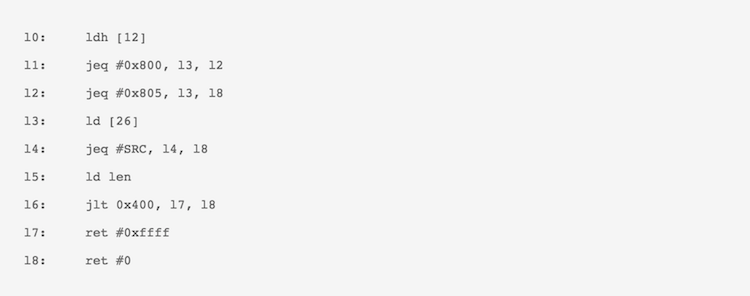
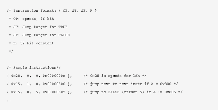
To know how to read these BPF instructions, look at the filter documentation in Kernel source and see what each line does. Each of these instructions are actually just bytecodes which the BPF machine interprets. Like all real machines, this requires a definition of how the VM internals would look like. In the Linux kernel’s version of the BPF based in-kernel filtering technique they adopted, there were initially just 2 important registers, A and X with another 16 register ‘scratch space’ M[0-15]. The Instruction format and some sample instructions for this earlier version of BPF are shown below:
There were some radical changes done to the BPF infrastructure recently – extensions to its instruction set, registers, addition of things like BPF-maps etc. We shall discuss what those changes in detail, probably in the next post in this series. For now we’ll just see the good ol’ way of how BPF worked.
Interpreter
Each of the instructions seen above are represented as arrays of these 4 values and each program is an array of such instructions. The BPF interpreter sees each opcode and performs the operations on the registers or data accordingly after it goes through a verifier for a sanity check to make sure the filter code is secure and would not cause harm. The program which consists of these instructions, then passes through a dispatch routine. As an example, here is a small snippet from the BPF instruction dispatch for the instruction ‘add’ before it was restructured in Linux kernel v3.15 onwards,
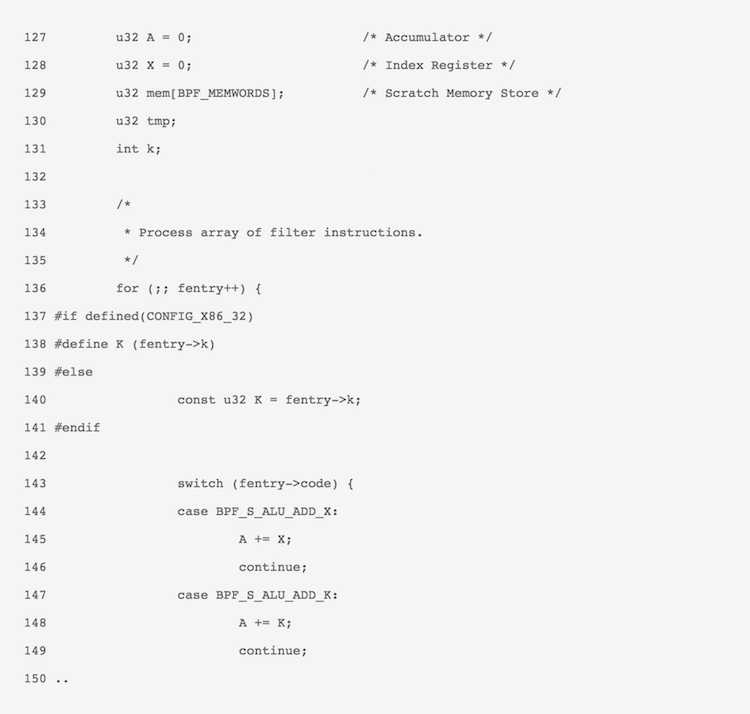
Above snippet is taken from net/core/filter.c in Linux kernel v3.14. Here, fentry is the socket_filter structure and the filter is applied to the sk_buff data element. The dispatch loop (136), runs till all the instructions are exhaused. The dispatch is basically a huge switch-case dispatch with each opcode being tested (143) and necessary action being taken. For example, here an ‘add’ operation on registers would add A+X and store it in A. Yes, this is simple isn’t it? Let us take it a level above.
JIT Compilation
This is nothing new. JIT compilation of bytecodes has been there for a long time. I think it is one of those eventual steps taken once an interpreted language decides to look for optimizing bytecode execution speed. Interpreter dispatches can be a bit costly once the size of the filter/code and the execution time increases. With high frequency packet filtering, we need to save as much time as possible and a good way is to convert the bytecode to native machine code by Just-In-Time compiling it and then executing the native code from the code cache. For BPF, JIT was discussed first in the BPF+ research paper by Begel etc al. in 1999. Along with other optimizations (redundant predicate elimination, peephole optimizations etc,) a JIT assembler for BPF bytecodes was also discussed. They showed improvements from 3.5x to 9x in certain cases. I quickly started seeing if the Linux kernel had done something similar. And behold, here is how the JIT looks like for the ‘add’ instruction we discussed before (Linux kernel v3.14),
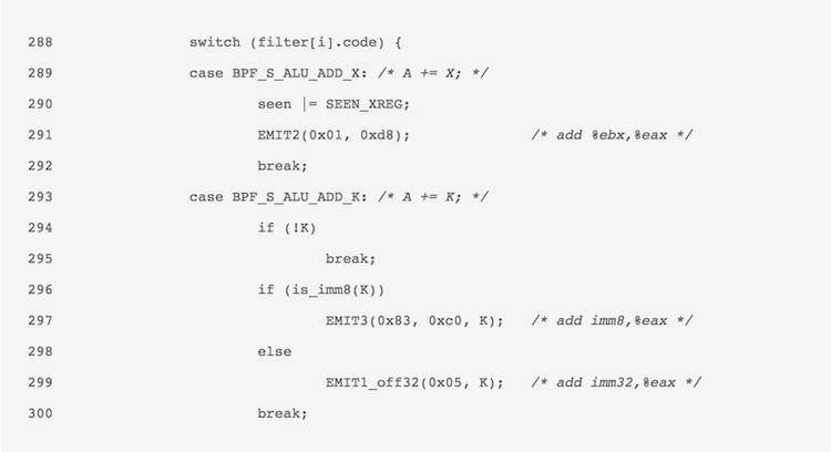
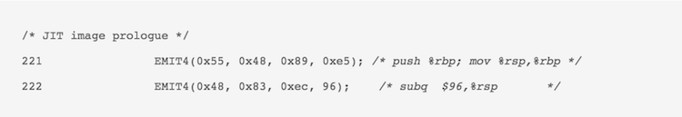
As seen above in arch/x86/net/bpf_jit_comp.c for v3.14, instead of performing operations during the code dispatch directly, the JIT compiler emits the native code to a memory area and keeps it ready for execution.The JITed filter image is built like a function call, so we add some prologue and epilogue to it as well,
There are rules to BPF (such as no-loop etc.) which the verifier checks before the image is built as we are now in dangerous waters of executing external machine code inside the linux kernel. In those days, all this would have been done by bpf_jit_compile which upon completion would point the filter function to the filter image,

Smooooooth… Upon execution of the filter function, instead of interpreting, the filter will now start executing the native code. Even though things have changed a bit recently, this had been indeed a fun way to learn how interpreters and JIT compilers work in general and the kind of optimizations that can be done. In the next part of this post series, I will look into what changes have been done recently, the restructuring and extension efforts to BPF and its evolution to eBPF along with BPF maps and the very recent and ongoing efforts in hist-triggers. I will discuss about my experiemntal userspace eBPF library and it’s use for LTTng’s UST event filtering and its comparison to LTTng’s bytecode interpreter. Brendan’s blog-post is highly recommended and so are the links to ‘More Reading’ in that post.
Thanks to Alexei Starovoitov, Eric Dumazet and all the other kernel contributors to BPF that I may have missed. They are doing awesome work and are the direct source for my learnings as well. It seems, looking at versatility of eBPF, it’s adoption in newer tools like shark, and with Brendan’s views and first experiemnts, this may indeed be the next big thing in tracing.
—
About the author of this post
 Suchakra Sharma